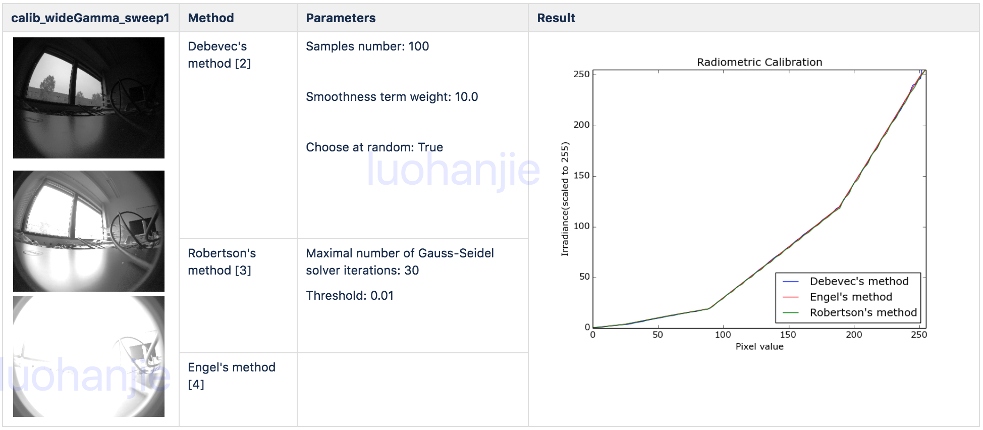
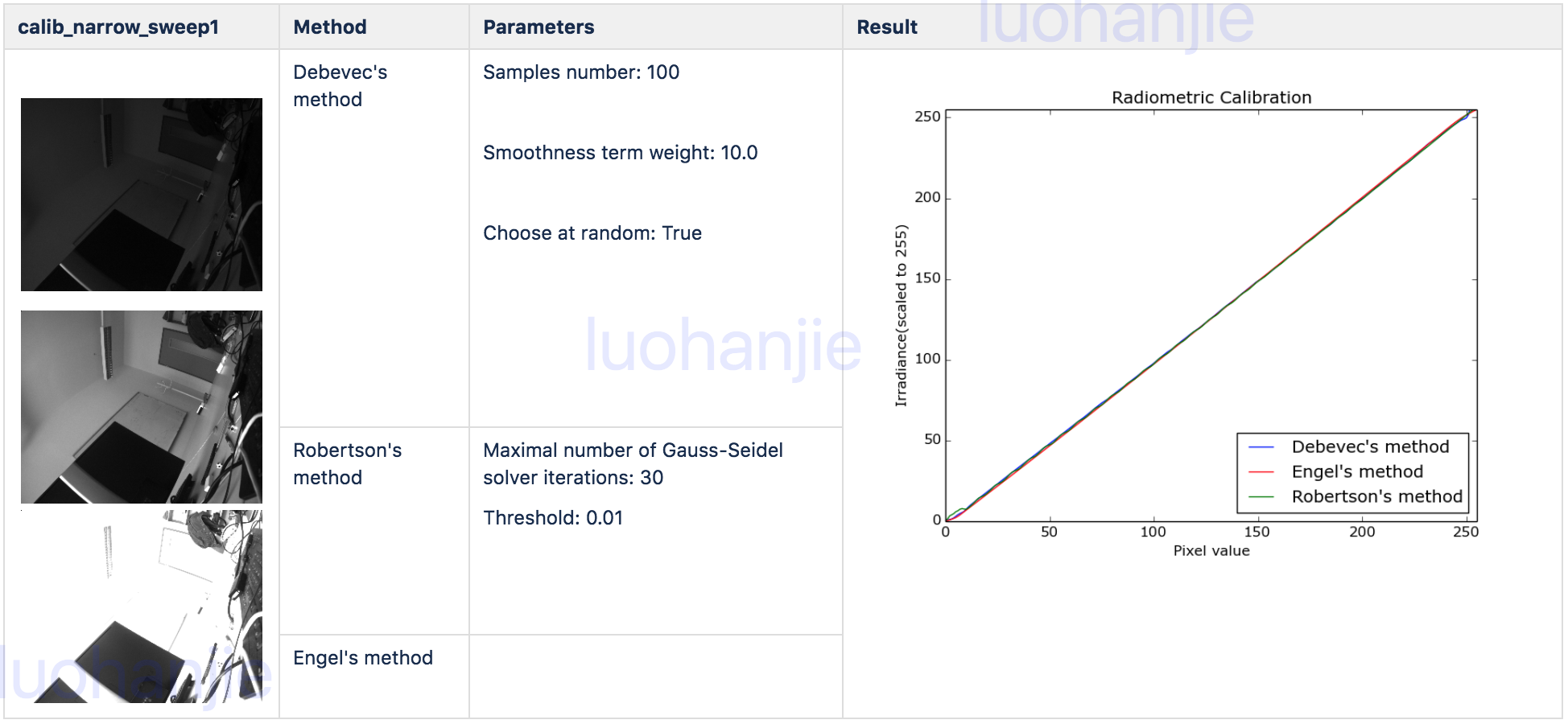
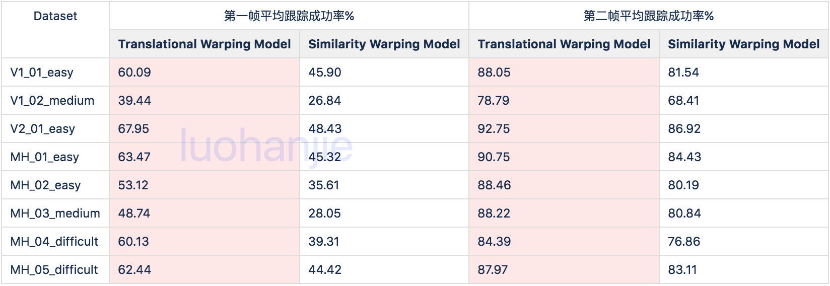
We compare the estimates resulting of TUM Mono VO dataset1 from algorithms proposed in 2 , 3 and
in 4 .
method comparision1method comparison2
As can be seen above, there is no significant difference between
methods. Engel's method performs better for the marginal values as
overexposed pixels are removed from the estimation. In this case,
Engel's method is selected for radiometric calibration.
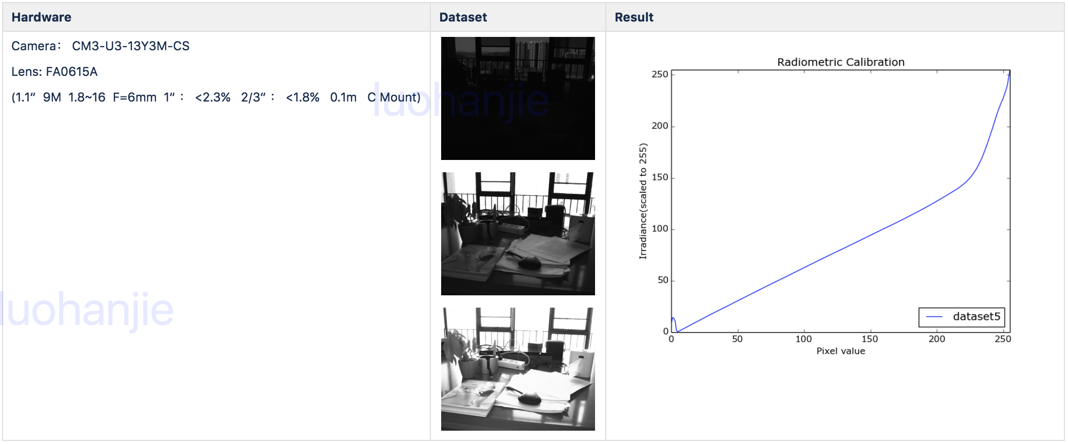
Radiometric
Calibration for Point Grey Camera
Radiometric Calibration1
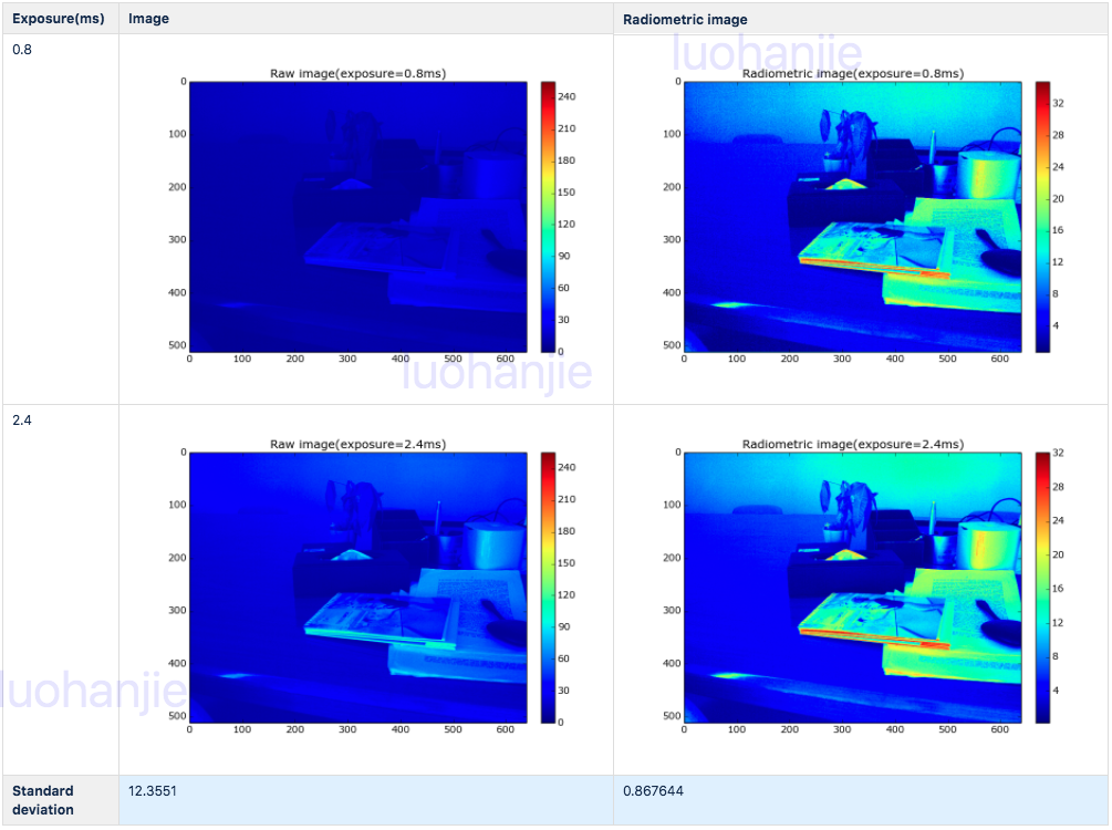
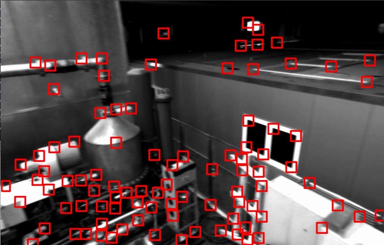
Experimental Verification
Evaluation in static
environment
Radiometric image is obtained by recovering exposure time and inverse
radiometric response function for raw image. Two images are captured
taken under different exposures while the camera and the scene is fixed.
The radiometric images are computed accordingly after that.
Radiometric Calibration2
Experiment shows that the recovering image irradiance stay stable
regardless of exposure change.
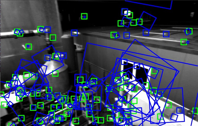
Evaluation in dynamic
environment
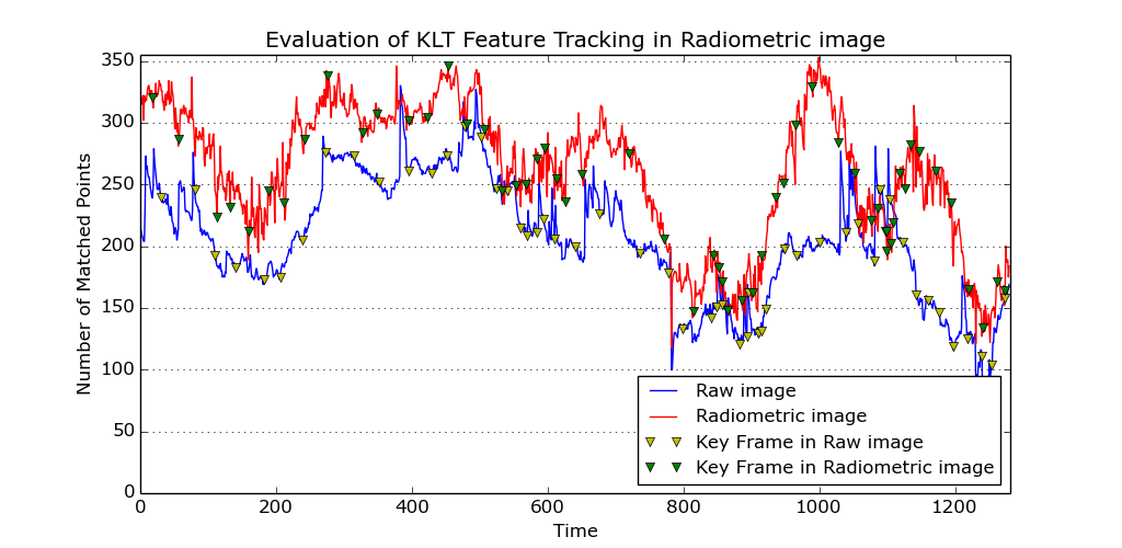
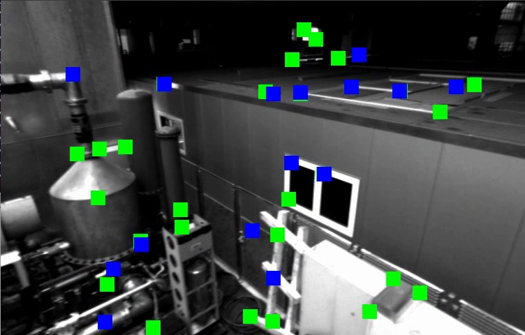
Evaluation
of KLT Feature Tracking in Radiometric image
Validation
The experiment above compares the number of matching feature points
in the radiometric image and in the raw image on indoor scene.
Debevec, P.E. and Malik, J., 2008, August. Recovering
high dynamic range radiance maps from photographs. In ACM SIGGRAPH 2008
classes (p. 31). ACM.↩︎
Robertson, M.A., Borman, S. and Stevenson, R.L., 1999.
Dynamic range improvement through multiple exposures. In Image
Processing, 1999. ICIP 99. Proceedings. 1999 International Conference on
(Vol. 3, pp. 159-163). IEEE.↩︎
Engel, J., Usenko, V. and Cremers, D., 2016. A
photometrically calibrated benchmark for monocular visual odometry.
arXiv preprint arXiv:1607.02555.↩︎
Hwangbo M, Kim J S, Kanade T. Inertial-aided KLT feature
tracking for a moving camera[C]//Intelligent Robots and Systems, 2009.
IROS 2009. IEEE/RSJ International Conference on. IEEE, 2009:
1909-1916.↩︎
Hwangbo, M., Kim, J.S. and Kanade, T., 2011. Gyro-aided
feature tracking for a moving camera: fusion, auto-calibration and GPU
implementation. The International Journal of Robotics Research, 30(14),
pp.1755-1774.↩︎
Chermak, L., Aouf, N. and Richardson, M.A., 2017. Scale
robust IMU-assisted KLT for stereo visual odometry solution. Robotica,
35(9), pp.1864-1887.↩︎